Category Archives: C/C++/Embedded

Code Kata 4: Struct Member Alignment

“The whole is greater than the sum of its parts”
— Aristotle

How time flies! More than two years have passed since I posted my last kata, so it’s high time for a new one. Today’s kata is based on a real problem that I had to solve last week when I worked on a code generator that produced C/C++ code. I hope you enjoy this task as much as I did!

When you define a struct in C, the overall size of the struct is not necessarily the sum of its members. Much like in real life, the whole is greater than the sum of the parts. Consider this example:

Only novice programmers would assume that sizeof(Foo) equals 5; experienced programmers know that 8 is a much safer bet. How come?

Most computer architectures can access data only if it is properly aligned in memory, e. g. a 32-bit (4-byte) integer can only be accessed if it is stored at an address that is evenly divisible by 4. The compiler usually achieves this by inserting invisible padding bytes between the struct members. Thus, internally, struct Foo is likely to look like this:

As a first step, familiarize yourself with struct padding. Check out this must-read by legendary Eric S. Raymond, especially if you are a systems programmer.

Now that you have read it, you should understand why sometimes there is also trailing padding (but never leading padding) and hence why the size of the following struct is most likely 12:

Equipped with this knowledge we are ready to tackle our first programming task: assume that every primitive struct member of base-2 size is to be aligned on its base-2 boundary (a 2-byte integer on an address that is evenly divisible by 2, a 4-byte integer on an address that is evenly divisible by 4 and so on). Implement an algorithm that computes the overall size of a struct given an ordered list of its members. Instead of real types, provide a list of integer values where the values represent the sizes of the members. Here are examples for Foo and Bar (in Python):

One weakness of this approach is that you cannot differentiate between a unit32_t (size is 4, alignment is 4) and an array of 4 uint8_ts (size is 4, alignment is 1):

Extend your algorithm to accept a list of pairs, where the first pair member specifies the size and the second pair member specifies the alignment:

But there is one more feature we need to add before we’re done: support for arbitrarily nested structs:

How does a member that itself is a struct impact the alignment of the outer struct? Devise a suitable data structure for passing in nested struct specifications.

[Update 2016-03-12: I’ve uploaded a sample solution to GitHub]

So long Scott Meyers, So long C++?

Last month, Scott Meyers wrote a blog post where he announced that he will withdraw from active involvement in C++.

Scott is famous for at least two things: first, his excellent way of explaining dry technical stuff in an entertaining way (I read all his books on C++, except for “Effective Modern C++” which is still on my to-be-read pile) and second, his He-man like hairdo.

After 25 years of dedicating his life exclusively to C++ he has become tired — tired of a language that gets more and more complex at an seemingly ever-increasing rate, all in the name of backwards compatibility and efficiency. (He didn’t say that, but this is my view.)

Ah, speaking of efficiency, the “e” word.

Just because C++ gives you control over efficiency doesn’t mean that you will get it in the end. Due to a lack of compiler and hardware knowledge, many C++ developers have a wrong (insufficient, at least) notion about efficiency. There are many misconceptions, because they don’t know how compilers, CPUs, or memories work.

One example is not understanding the effects of caching. Many C++ developers blindly trust std::map’s or std::unordered_map’s O(log n) and O(1) promises but there are situations where an O(n) std::vector (or plain C-style array) can be orders of magnitude faster because it accesses memory in a cache-friendly way. There is a nice talk by Scott on YouTube where he gives a good overview about caching and its consequences.

Another common efficiency fallacy is illustrated by this little for loop:

Many developers I’ve met believe that using a ‘uint8_t’ for the loop counter is more efficient than using a plain ‘int’. But what most likely will happen is that by using ‘uint8_t’ the code becomes both, bigger and slower, especially on modern RISC-style processor architectures like ARM and PowerPC. Why? If the value of ‘arrayLength’ is not known at compile-time, the compiler has to create additional code that ensures that ‘i’ wraps around for values greater or equal to 256. Internally, the compiler assigns a 32-bit register to ‘i’ (provided you are targeting a 32-bit platform) and adding 1 to 255 in a 32-bit register is different to adding 1 to 255 in an 8-bit register. Behind the scenes, your compiler rewrites your loop to look like this:

Granted, in most situations this additional code will not amount to much, but maybe in a low-level driver or some communications stack, situations which systems languages like C++ were made for. But this example shows a problem that many would-be efficiency experts share: for the sake of (false) efficiency, they increase complexity and risk correctness and security. What happens if some day ‘arrayLength’ can be larger than 255? The for loop will loop forever, of course.

So while C++ is a language that has the potential to yield extremely efficient systems, you neither get efficiency automatically nor for free. C++ has a steep learning curve and there are many pitfalls. I truly belief that much of C++’s efficiency is wasted on too many developers. If you don’t need utmost efficiency or don’t know how to put the corresponding language features to best use, better keep away from C++ and use a managed language. You will be much more productive and create programs that are also (probably) more secure by default.

Getting back to Scott Meyers, I must admit that I’m somewhat happy about his decision. Not because he left C++ per se but because he now has time to focus on other important topics — topics that he will explain with the same quality he is renowned for. Like some programmers say: when one curly brace closes, another one opens.

Circular Adventures VI: When the Winner is Known Beforehand

“Girls have an unfair advantage over men: if they can’t get what they want by being smart, they can get it by being dumb.”
— Yul Brynner

In part III and IV I discussed solutions for a circular problem where two indices performed a race within a circular buffer; that is, either index could be ahead of the other.

Sometimes, however, life is simpler and it is always known which index is the leader, and thus the winner — from the outset:

In this example, provided we know that b must always be ahead of a, we can deduce that b has wrapped around and the distance between a and b is 4.

Either implementation (the one given in part III and the one given in part IV) of circular_distance will return the same result:

However, both will fail for this case:

Why? Under the premise that b is always ahead of a, the distance is +6 not -4. circular_distance computes the wrong result because it assumes that the leading index is less than half the circular buffer size ahead of the other index. This assumption was made (I called it ‘invariant’ at the time) to be able to compute the circular distance even if it is not known which index is ahead of which.

Based on the prerequisite that b is always ahead of a we can give a simplified version of the circular_distance function from part III:

I call this function circular_lead instead of circular_distance to emphasize that it returns how much b is ahead of a, which is always a positive number. As usual, all the restrictions (and optimizations) regarding the mod operator apply. In C, which lacks a true mod operator, a generic, portable implementation looks like this:

In situations where one index is known to be ahead of the other, circular_lead has an edge over circular_distance because it supports distances in the range 0 to N-1, whereas circular_distance only supports ranges from 0 to (N-1)/2. This is always the case in “monotonically increasing” scenarios, like run-time measurement, at least until the flux capacitor is invented. Hence, the last example of part IV can be rewritten like this:

If we replace the mod operator with a cast to uint32_t, circular_lead_32bit boils down to this:

[For the mathematically inclined: What we are really talking about here is residue class rings, a concept used by all contemporary computers. I might explore the number theory behind this and other circular topics in a future post.]

More circular adventures…

Bug Hunting Adventures #9: A Random Piece of PI

According to an old saying, there’s more than one way to skin a cat. There are at least as many ways to compute the value of Ï€. One of them uses the Monte Carlo method to approximate Ï€’s value and it is the subject of today’s Bug Hunting epsisode.

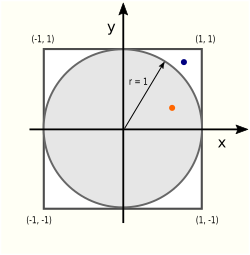
We start with a so-called unit circle, a circle with radius 1 whose center is positioned at the origin in the Cartesian coordinate system. Next, we put a square around the unit circle whose sides have length 2 (the diameter of the unit circle):

drawingThere are two areas (literally!) of interest in this picture: the circle area Ac and the square area As:

Ac = πr² = π
As = (2r)² = 4

The ratio Ac/As is π/4

Why is this ratio important? Because we can use it to calculate the value of π:

Ï€ = 4 Ac/As

Now let’s do some random sampling. We take N random points whose x and y values are both in range [-1; +1] and tally the number of points that fall within the square (Ns) and the number of points that fall within the circle (Nc). Given enough points, the ratio Nc/Ns is a very good approximation for Ac/As and we hence can compute:

π ≈ 4 Nc/Ns

The C code below attempts to calculate π in this manner, but sports a blunder. What is the bug? Bonus question for the mathematically inclined: without executing the code, what value does it really compute (instead of π)?

Code
Solution

Bug Hunting Adventures #8: Just Like a Rubber Ball…

Two incidents gave rise to this Bug Hunting episode: first, I’m currently beefing up my burglar alarm system with a Raspberry Pi and second, I’ve just come across the old song from the ’60s “Rubber Ball” by Bobby Vee while randomly surfing YouTube (“Bouncy, bouncy, bouncy, bouncy”).

The alarm system extension I have in mind is this: I want to be able to configure temporary inhibition of motion detection via a simple push-button: if you press it once, you suppress motion detection by one hour, if you press it n times, you suppress it by n hours, respectively. If you press the button after you haven’t pressed it for five seconds, any suppression is undone. There are status LEDs that give visual feedback such that you know what you’ve configured.

Thanks to the fine RPi.GPIO library, accessing GPIO ports is usually a piece of Pi. However, there is a fundamental problem when reading digital signals from switches and buttons called “switch bounce”, a phenomenon that has driven many brave engineers nuts.

If you flip a switch, there never is a nice transition from zero to one (or one to zero, depending on how you flipped the switch). Instead, the signal bounces between zero and one, in a rather indeterminate fashion for many milliseconds. The bouncing characteristics depend on various factors and can even vary for the same type of switch.

The takeaway is this: with switches (and buttons, of course), expect the unexpected! You must use some sort of debouncing mechanism, implemented in either hardware or software. For some background information check out this excellent article by embedded systems luminary and die-hard veteran Jack Ganssle.

But back to my alarm system. I skimmed the RPi.GPIO documentation and was happy to read that since version 0.5.7, RPi.GPIO has support for debouncing of digital input signals, so there was no need to debounce the push-button myself. Exuberantly, I sat down and wrote this test code:

To avoid arbitrary, floating input voltages, I setup the port such that it is pulled down (to ground) by default. As a consequence, reading that port when the button is not pressed yields a clean zero.

I didn’t want to poll the button port, as this would burn valuable CPU cycles, so I registered an event handler with the RPi.GPIO library that would be called back once a rising edge had been detected. I added a ‘bouncetime’ parameter of 200 milliseconds, to avoid multiple calls to my ‘button_pressed’ handler, in full accordance with the RPi.GPIO documentation:

To debounce using software, add the ‘bouncetime=’ parameter to a function where you specify a callback function. Bouncetime should be specified in milliseconds. For example:

In other words, after a rising edge has been detected due to a button press, I won’t be bothered with spurious rising edges for 200 ms. (200 ms is plenty of time — no switch I’ve ever seen bounced for more than 100 ms. Yet, 200 ms is short enough to handle cases where the user presses the button in rapid succession.)

I tested my button for a minute and it worked like a charm; then, I varied my press/release scheme and suddenly some spurious “Button pressed!” messages appeared. After some head scratching, I discovered the problem — can you spot it, too? (Hint: it’s a logic error, not something related to misuse of Python or the RPi.GPIO library.)

Epilogue: Once the problem was understood, the bug was fixed easily; getting rid of this darn, “bouncy, bouncy” earworm was much harder, though.

Solution

Bug Hunting Adventures #7: Random Programming

If you want to draw m random samples out of a set of n elements, Knuth’s algorithm ‘S’ (ref. The Art of Computer Programming, Vol 2, 3.4.2) comes in handy. It starts out by attempting to select the first element with a probability of m/n; subsequent elements are selected with a probability that depends on whether a previous element was drawn or not.

Let’s do an example. To select 2 random samples out of a set of 5 (say, the digits ‘0’, ‘1’, ‘2’, ‘3’, and ‘4’), we select ‘0’ with a probability of 2/5. If ‘0’ is not chosen, we attempt to select ‘1’ with a probability of 2/4 (since there are only 4 candidates left); otherwise (if ‘0’ has been selected) with a probability of 1/4, since one attempt to draw has already been used up. It’s easy to show the corresponding element selection probabilities in a binary tree:

In this tree, the nodes represent the likelihood that the element in the column on the right will be picked. Transitions from a node to the right mean that the element was picked, while transistions to the left denote that the corresponding element was not picked. In the ‘selected’ case, the numerator is decreased by one; the denominator is decreased in either case.

Here is an implementation of Knuth’s algorithm in C:

For the sake of demonstration, assume that bigrand() is a function that returns a random number that is “big enough”, meaning a value that is greater or equal to 0 and has an upper bound of at least n – 1 (a larger upper bound does not harm). Spend some time to understand how the ‘if’ statement implements the selection with the correct probablity.

So far, so good. But how would this clever algorithm look in another language? Let’s port it to Ruby!

Not being a Ruby programmer (but being an experienced Online Programmer), I had to ask Auntie Google many questions in order to cobble together this code:

This Ruby code looks remarkably similar to the C version. It doesn’t contain any syntax errors, but nevertheless doesn’t output what it is supposed to. Can you see why?

For those folks who don’t want to waste their time on Ruby, here is the Python version, sporting the same behavior and thus the same blunder:

Solution